RATTACA results

I just received my RATTACA results. What do I do with them?

RATTACA requests fall under two main categories: “standard” requests (for predictions and samples of extreme rats from the most recent colony cohort) and “ad-hoc” requests (for predictions on a desired sample of previously-genotyped rats). Depending on the details of your request, you will receive a number of different results files, and the results from either differ slightly. Here we provide general walkthroughs for interpreting results from either request type. Any details specific to your request will be provided to you with your data.

Standard RATTACA

Predictions file: rattaca**results**.csv

Your primary RATTACA results are provided in a csv file named following the format ‘rattaca’ + colony generation + ‘results’ + investigator + primary trait or paradigm of interest. So, for Dr. Splinter’s request for ninja-related trait predictions from generation 100 rats, this file would be named rattaca_gen100_results_splinter_ninja_rats.csv.

Here is a walkthrough of standard metadata columns and their interpretation:

• rfid: This is a given rat’s RFID transponder identifier, inserted subcutaneously in the rat’s nape and scannable using an RFID microchip reader.
• rfid_orig: In rare cases, a rat’s original RFID chip (inserted at the time of weaning) may fall out, requiring insertion of a new one at the time of shipment for your order. Your rats all have RFIDs from the rfid column, but this column is provided just in case.
• generation: The RATTACA generation from which a given rat was derived.  
• animalid: This is the colony ID used for a given rat in the HS West colony. All animal IDs are unique with a 1:1 mapping to a rat’s RFID.
• earpunch: This is the earpunch pattern visible on each given rat, where R = right ear, L = left ear, B = bottom edge, T = top edge, M = middle edge, and C = center of the ear.
• sex: The phenotypic sex of the rat.
• coatcolor: The rat’s coat color pattern.
• dob: The rat’s date of birth.
• dow: The rat’s date of weaning (separation from the mother).
• comments: Any colony-related comments specific to the rat.

All subsequent columns include your actual RATTACA data! There are four columns per trait requested. Using the trait ‘super_stealth’ as an example:

• super_stealth: The column with the raw trait name shows the “raw” predicted trait value for each rat. This could alternatively be termed the polygenic score, polygenic index, polygenic risk score, or genomic estimated breeding value in different fields. Ultimately, this value reflects the cumulative genetic contribution (the sum of effect sizes) of all sampled genetic variants to the phenotype in each rat.
  • Note: The units in this column are not the same as those of the actual trait, rather they are units of  z-scored “trait residual” following pre-processing of raw phenotype measurements used for GWAS analysis. As such, these raw predictions are not of particular interest per se. Rather, RATTACA is concerned with the relative values for each rat and where they fall within the distribution of predictions in the total sample.
• super_stealth_rank: This column stores the rank order of each rat’s polygenic score in this cohort’s total sample of RATTACA rats. (This cohort sample size will vary between generations. It is provided in the summary csv file outlined below).
  • Note: Rank correlates with the actual predicted value, so a rank of 1 reflects the smallest polygenic score in the sample. As an intuitive example, if we were predicting body size in a sample of 100 rats, the animal with the smallest predicted mass would be ranked 1 and the animal with the largest prediction would be 100. Ranking is not a biological interpretation of the trait prediction (i.e., rank 1 is not a “top” ranked prediction). For example, in the Olympics a 1st-place sprinter finished with the smallest time value in the population of racers, and a 1st-ranked weightlifter finished with the largest weight value in the population. If these values were RATTACA predictions, the sprinter’s score would receive the lowest rank and the weightlifter would receive the highest rank.
• super_stealth_zscore: This column stores the z-score for each rat’s prediction in the current RATTACA cohort. These values are perfectly correlated and statistically interchangeable with the raw predictions, and they are useful in helping to quickly identify rats with extreme predicted values. z-scores are in units of standard deviation, so a z-score of 0 reflects an animal at the population mean, 1 is an animal 1 SD above the mean, -1 is 1 SD below, etc. The larger the absolute value, the more extreme the prediction. Because these are standard scores, they are also useful for comparing to z-scores from other traits, even if they were measured with different raw units.
• super_stealth_group: This column classifies each rat as belonging to either a “high” or “low” sample for the trait of interest, defined by whether their polygenic score falls above (high) or below (low) the population median. Use these classifications to distinguish between your experimental samples of (predicted) phenotypically extreme rats. As with trait ranks, note that these groupings do not reflect any interpretation of the polygenic score, only their relative location in the population distribution.
  • Note: These classifications are obviously critical for making statistical comparisons between samples following experiments and data collection. However, we recommend ignoring them prior to analyses! We suggest blinding yourself to these classifications when setting up and conducting experiments to avoid any potential biasing during data collection.

Assignment plots: rattaca**assignment**.png

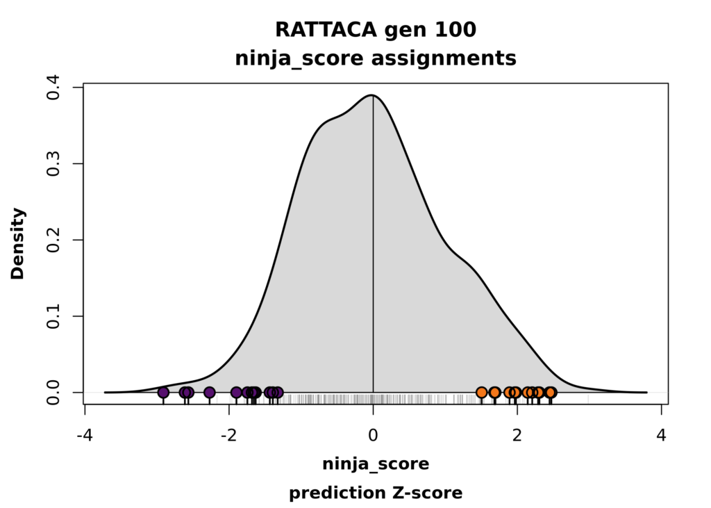
While RATTACA can provide predictions for any number of desired traits, we can only assign rats (decide which rats to send to an investigator) based on their predictions for one trait (for now, though with some workarounds – see below). As such, your results include two versions of RATTACA “assignment plots” for the trait used to assign your rats. The information content of both is the same: the distribution of trait predictions across the whole RATTACA cohort and where your individual rats fall within that distribution.

The first plot shows the density of trait predictions in standard (z-score) units. The base of the plot shows a “rug” of gray tick marks noting the values of all individual predictions in the total cohort. Your assigned rats are highlighted with bold black ticks and colored points to distinguish between high (orange) and low (purple) group assignments in your sample.
– Note: The goal of RATTACA is to provide you with samples of rats that are expected to statistically differ in the predicted trait of interest. If you ordered, say, 24 rats (meaning 12 high and 12 low for a specific trait), this would optimally entail assign to you all 24 of the most extreme rats from the current cohort. As in the figure below, in some cases you may notice from your assignment plot that your samples do not include all of the 12 most extreme rats from either end of the distribution. This is expected in some cases: if multiple investigators request assignments for the same or correlated traits, conflicts over assignments must be resolved using a tiebreaking algorithm. Each request is allotted a maximally-extreme sample (within constraints imposed by other projects) that is still expected to produce statistically distinct sub-samples.

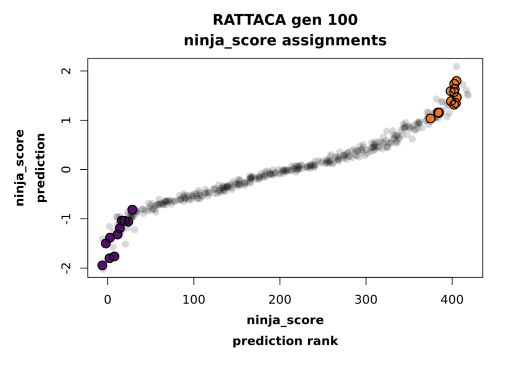
The second assignment plot displays the rank order of all predictions for your assigned trait versus the raw predictions (or PGSs) in the complete cohort, again with your high and low assigned rats highlighted in orange and purple, respectively. Note that this plot is jittered for visualization purposes, so the coordinates of each point aren’t exactly precise. Rest assured that the data in your predictions file are the real values!

Prediction correlations: rattaca_[generation]_[request]_corrplot.png

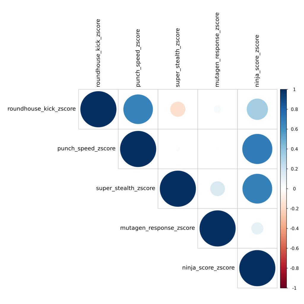
For requests involving predictions on multiple traits, we provide a correlation plot showing pairwise correlations between the z-scores of all requested traits. This is accompanied by the data used to produce the figure, named similarly to the file rattaca_gen100_ninja_rats_corr.csv. Note that these are correlations across the entire RATTACA cohort, not just your provided sample. Visualizing these correlations should help you quickly characterize how extreme your assigned sample is for other traits of interest in addition to the trait used for assignment.

Model performance summary: rattaca_[generation]_[request]_all_traits_summary.csv

This file displays basic summary stats about model performance in producing your predictions for all requested traits. Briefly, to get predictions we estimate the genetic effect size of individual genome-wide SNPs on phenotypes that have already been measured (termed the “training set”). These effect sizes are then used to predict trait values in naive rats without phenotype measurements (the “test set”). We can’t directly know the accuracy of your predictions as we don’t have true measurements to compare them to. However, we can get a general sense for the accuracy of our predictive model using k-fold cross validation. Here, we conducted a 5-fold cross-validation, meaning we trained 5 models, each on a different subset of phenotyped rats, and tested the accuracy of predictions on the remaining subset (the “validation set”) by comparing observed and predicted phenotypes. The summary statistics “r_sq”, “r”, and “rho” reflect this performance accuracy. Think of them as reflective of how well the model used for predictions here is generally expected to perform when predicting on new data. It is not an exact reflection of prediction accuracy in your sample, but is a ballpark expectation of what it could be. The columns in this summary file are:

• trait: The name of the trait used for predictions.
• generation: The RATTACA generation used as the test dataset
• heritability: The SNP-based heritability of the trait in the training set (the complete set of rats for which the Palmer lab has both trait and genotype data). This was calculated as part of prior GWAS analyses on the trait.
• n_train: The number of rats in the training set used to parameterize your predictions. This varies by trait.
• n_test: The number of samples in the test set, or the total number of rats on which predictions were made. This number reflects all animals in the RATTACA generation from which your assigned rats were sampled. Note that while your actual predictions and group assignments are specific to a subset of animals, these summary statistics reflect model performance across the entire cohort sample of n_test rats. 
• n_snps: The number of single nucleotide polymorphisms used in genomic prediction. Briefly, more SNPs tend to produce better prediction results, but at the cost of computational efficiency. We’ve found ~10k SNPs to be the inflection point above which model accuracy usually plateaus, and increasing SNP samples produce diminishing returns in prediction model performance. In RATTACA, we “LD-prune” our genome-wide sample of >7M SNPs before prediction. That is, we scan for pairwise linkage disequilibrium (LD) across the genome and retain one variant per LD block for our genomic training dataset. This approach maximizes genome-wide sampling of independent variants contributing to phenotypic variation while minimizing sample redundancy and computation costs.
• mean_r_sq: The mean coefficient of determination (r²) calculated across the 5 folds of the cross-validation analysis, where r² is defined as the proportion of variation in predicted trait values that was predictable by the trait measurements.
• mean_r: The mean Pearson correlation coefficient of the cross-validation analysis, estimated between measured and predicted trait values in each validation set.
• mean_rho: The mean Spearman rank correlation of the cross-validation analysis, estimated between measured and predicted values each validation set. Whereas the Pearson correlation reflects the correlation in raw trait scores and measurement, the Spearman correlation is that between their rank orders. Because RATTACA is mostly interested in trait ranks (not absolute trait values), this might be a more relevant demonstration of model accuracy.
• description: This is taken from a data dictionary provided by external collaborators, where available. We in the RATTACA team are not experts in behavioral experimental paradigms or in the biological interpretation of these traits, so we provide an outside expert’s description of each for reference. 
• covariates: This lists the covariates used when pre-processing the trait prior to polygenic prediction. Items in this list represent covariates with sufficient contribution to variance in the raw phenotype that their variance was removed using a linear model prior to prediction. This pre-processing is a standard part of RATTACA (1) to maintain prediction model simplicity across different traits and (2) to ensure all polygenic scores reflect only the genetic contribution to the trait.
• variable_used: This shows the file and full variable name used in assembling the phenotypic training data. Predicted trait names used here are truncated for ease of interpretation (and coding), but we provide these full names here so nobody forgets where exactly the data came from and so traits don’t get forgotten in translation.
• source_file: This is the complete file path (on the UCSD computing cluster used by the Palmer lab) to the phenotype dataset used for model training. Depending on the trait, many of these datasets are updated regularly, this is a pointer to the exact copy used at the time your predictions were made. You likely do not need this information, but it will be helpful to provide it back to us in the event you wish to revisit any analyses or data.

Composite traits: [composite_trait]_corrplots.png

Because RATTACA can only assign rats based on one trait, some investigators may opt to construct a “composite” trait from multiple traits’ predictions, then use this composite for assignment. This is highly context-dependent and will require detailed discussions of desired traits (and their interpretations) prior to prediction, but his strategy can help identify rats that consistently meet multiple desired criteria for assignment.

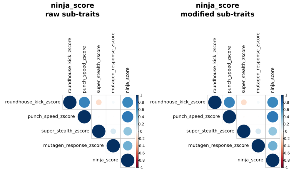
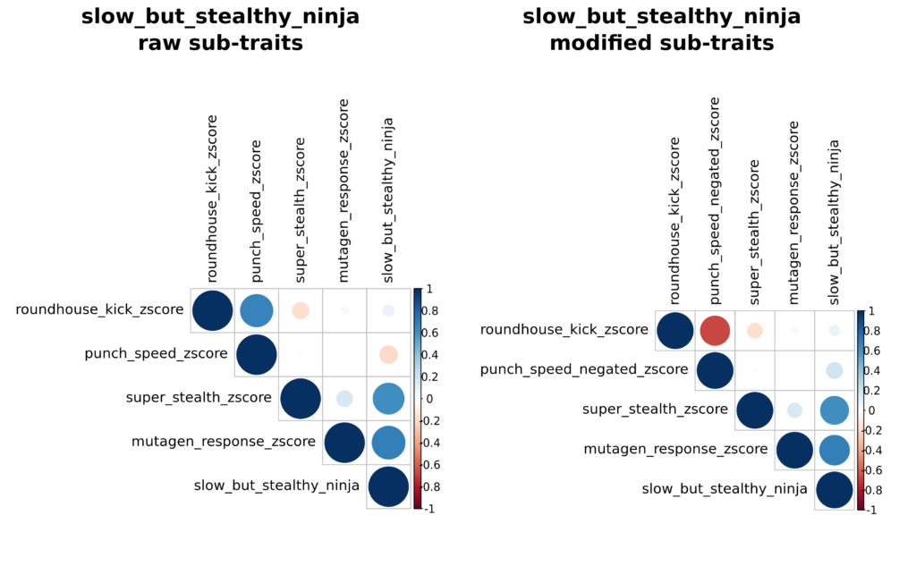
In our example using Dr. Splinter’s traits, roundhouse kick strength, punch speed, super stealth, and response to mutagen are all traits that were measured experimentally and have data usable for prediction. Because Dr. Splinter was interested in rats that scored highly for all of these traits, he opted to use a composite score for all of them, which we termed ninja_score. This composite “trait” is constructed after predictions, using prediction z-scores as inputs, by taking the simple mean of the z-scores for each trait for a given rat. These composite scores are then rank-ordered for assignment as usual. To interpret this trait, an extremely high composite score reflects rats that are on average high in the four desired sub-traits and an extremely low ninja score reflects rats that have low predictions on average. Note that since this is not a “real” trait that is directly measured experimentally, there are no predictions associated with it. Results for composite traits are visualized in files named similarly to ninja_score_corrplots.png with two plots: one showing correlations between the raw, unmodified sub-traits and the final composite trait, and the second showing correlations between modified versions of the sub-traits used to calculate the composite trait. Because ninja_score did not require any modifications to sub-traits in this case, the two panels for this trait are identical. Accompanying data are available in ninja_score_corr_raw_traits.csv and ninja_score_corr_altered_traits.csv (again identical in this case). The actual composite scores (including ranks and z-scores) are provided in the file ninja_score_composite_scores.csv.

“Modified” composite traits

In the above ninja_score example, Dr. Splinter knew he wanted to use predictions from each sub-trait as-is, which identifies rats that are consistently high (or low) across all sub-traits. In some cases, an investigator may want to prioritize assigning rats that are predicted to be both extremely high for one trait and extremely low for another. RATTACA can accommodate these requests with composite traits that meet these variable criteria. For example, in addition to his desired sample of simple ninja_score rats, Dr. Splinter was also interested in testing rats that were predicted to be slow but still stealthy teenage mutant ninjas. To meet this request, we produced a composite trait that first “negates” punch speed by multiplying punch_speed z-scores by -1. This switches the orientation of the z-scores such that all sub-traits are re-aligned in a direction that positively correlates all desired trait values. When the average of sub-trait scores are taken, the resulting composite score produces extremely high values that are on average predicted high for all traits Dr. Splinter wished to maximize (roundhouse_kick, super_stealth, and mutagen_response), and extremely low in the desired trait to minimize (punch_speed). The modification can be visualized in the right panel of slow_but_stealthy_ninja_corrplots.png, both in the modified trait name and in the correlation between punch_speed and the composite score. Accompanying data are again provided in similarly-named csv files.

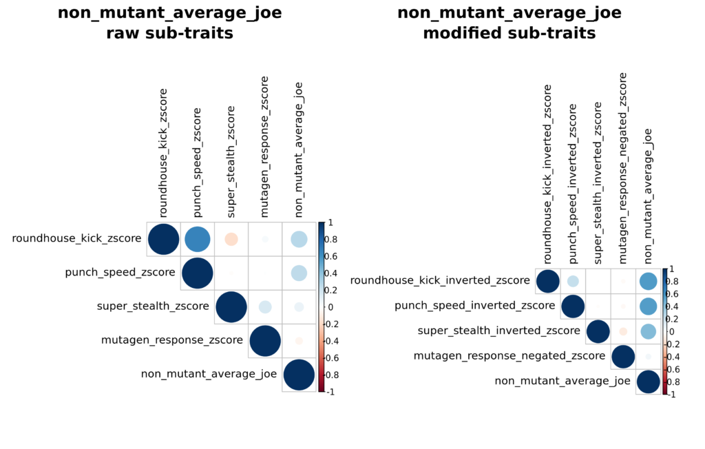
While RATTACA is generally used to identify predicted extreme trait values, in some cases investigators may desire rats with intermediate polygenic scores for a certain trait. As a relevant example, Dr. Splinter was also interested in receiving RATTACA rats that were least likely to display any teenage-mutant ninja phenotypes, i.e., “average joe” rats. To construct this composite trait, we negated predictions for mutagen_response (similar to punch speed above) to prioritize rats least likely to become mutants. We also “inverted” roundhouse_kick, punch_speed, and super_stealth z-scores by replacing each z-score with 1/z-score. This modification switches assignment priority from extreme to intermediate predictions such that originally small-magnitude z-scores become large and large scores become small, all without reversing the high vs. low group orientation of predictions introduced by negation. To interpret this trait, high values reflect those rats who on average show intermediate roundhouse kick strength, punch speed, and stealth predictions, and low responses to mutagen. Sub-trait modifications are visible in non_mutant_average_joe_corrplots.png and accompanying csv files:

ad-hoc RATTACA

Details coming soon!